
Crop Monitoring for Al Jouf Without a Server
Sentinel-2, an offline Python pipeline and a static WebGIS
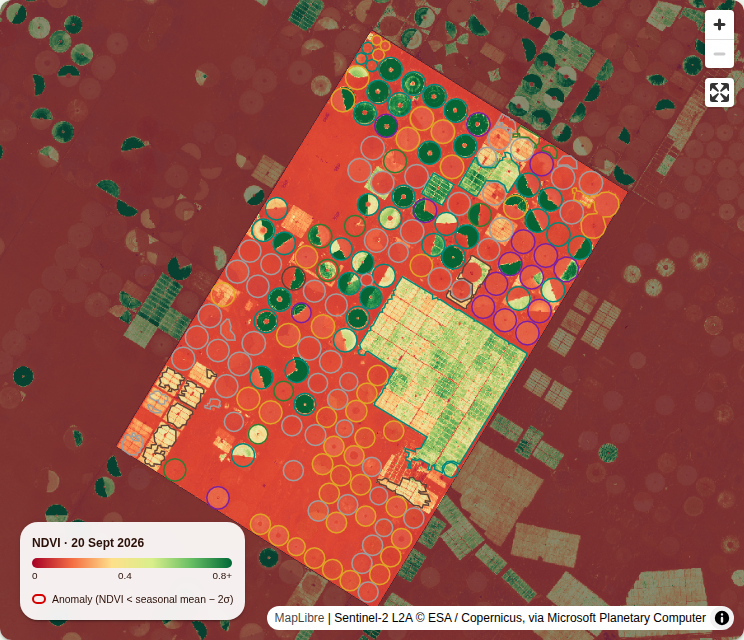
The dashboard finds 160 centre pivots and 21 block fields in Al Jouf automatically, covering 13,781 hectares, and follows every one through 442 Sentinel-2 scene dates since April 2023. Each field gets a crop type per season, and 50 fields have been flagged at least once for falling behind their peers. No server of mine runs at any point.
Open the GeoAI Crop Monitoring dashboard →
Why Al Jouf
Al Jouf in northern Saudi Arabia is one of the Kingdom's largest agricultural regions, known for its olive orchards as well as cereals and forage. From space it is unmistakable: rows of green centre-pivot circles in the desert, each one irrigated with groundwater.
That makes field-level monitoring useful to more than agronomists. What is grown, when, and whether a field is thriving tells you a lot about water use in one of the driest farming regions on Earth. The dashboard answers three questions for every field: what is growing, how is it doing, and is anything going wrong?
What it shows
| Measure | Value |
|---|---|
| Centre pivots detected | 160 |
| Block fields detected | 21 |
| Total field area | 13,781 ha |
| Sentinel-2 scene dates processed | 442 (April 2023 – September 2026) |
| Crop classes assigned | fallow, alfalfa / forage, orchard, double crop, winter cereal, summer crop |
| Fields flagged at least once | 50 (none on the latest date, 20 September 2026) |

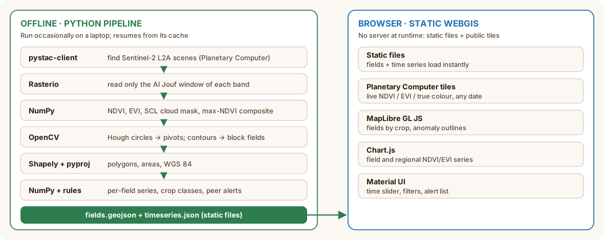
Two halves: an offline pipeline and a static WebGIS
My other browser-only projects, Blue Nile Flood Risk and Riyadh Urban Heat, compute everything live in the browser. Crop monitoring takes a different route, and the reason is scale: every Sentinel-2 scene since 2023 × every field is not something to recompute on each page view.
So the work is split in two:
- An offline Python pipeline that I run occasionally. It reads Sentinel-2 straight from the cloud, detects fields, computes time series, classifies crops and flags anomalies, then writes two static files:
fields.geojsonandtimeseries.json. - A static WebGIS that loads those files and streams live index tiles for any date from Planetary Computer's public tile API.
At runtime there is still no server of mine anywhere: static files on shared hosting, plus public, CORS-enabled tiles.
The pipeline (Python, offline)
| Library | Role |
|---|---|
| pystac-client | Searches the Planetary Computer STAC catalogue for Sentinel-2 L2A scenes |
| planetary-computer | Signs asset URLs so they can be read anonymously |
| Rasterio | Windowed reads of cloud-optimised GeoTIFFs over HTTP: only pixels inside the area are downloaded |
| NumPy | Vegetation indices, composites and statistics |
| OpenCV | Hough circle transform, morphology and contours to detect fields |
| Shapely and pyproj | Field geometries, reprojection and areas |
No imagery is downloaded in bulk. Rasterio reads just the window it needs from each cloud-optimised GeoTIFF, in parallel threads, and results are cached so the pipeline can resume where it stopped.
1. Finding the fields
The pipeline takes the clearest Sentinel-2 scene of each month (under 5% cloud), masks clouds and shadows with the Scene Classification Layer (SCL), and stacks them into a maximum-NDVI composite at 10 m. In that image, every pivot that was ever green is a bright disc.
Detection is classical computer vision in OpenCV, with no training data:
- a Gaussian blur, then
cv2.HoughCirclesproposes circles of 200–480 m radius; - each candidate must be green (NDVI > 0.4) over most of its disc, lie inside the area, and not overlap a pivot already kept;
- a rim-contrast test keeps only real pivots: green just inside the rim, bare desert just outside. Circles "found" inside gridded block farms fail it.
Vegetated land that isn't a pivot becomes block fields. Morphological opening and closing clean the mask, connectedComponentsWithStats keeps areas over 8 ha, and findContours with approxPolyDP turns each one into a polygon. Shapely and pyproj clip the fields to the area, compute their areas and convert them to WGS 84.
2. NDVI and EVI time series
For every scene date since April 2023 (reprocessed duplicates removed), each field gets its mean NDVI and EVI at 20 m, the resolution of the SCL cloud mask, masked pixel by pixel.
Instead of looping over fields, the fields are rasterised once into a label image, and np.bincount sums every field's pixels in one vectorised pass. Thousands of fields cost about the same as one.
Three details matter for correct values:
- The +1000 offset. From processing baseline 04.00 (January 2022), Sentinel-2 reflectances carry a +1000 offset that must be removed first. Forget it and every index is biased.
- Reflectance scale. EVI = 2.5 × (NIR − Red) / (NIR + 6 × Red − 7.5 × Blue + 1) only works with reflectance on a 0–1 scale, so values are divided by 10,000 after removing the offset. NDVI is a ratio and doesn't care.
- Why EVI too. EVI saturates less than NDVI over dense, irrigated canopies, which is exactly what a healthy pivot is.
A field-date value only counts if at least 60% of the field's pixels are clear.
3. Crop type from phenology
A rule-based classifier reads each field's 12 monthly maximum NDVI values for each agricultural season (September–August). It counts "green" months (NDVI ≥ 0.4) and separate green spells:
| Rule | Class |
|---|---|
| Peak NDVI below 0.3 | Fallow |
| Green for 8 months or more | Alfalfa / perennial forage |
| Moderate, flat NDVI all year | Orchard |
| Two green spells covering 5+ months | Double crop |
| Peak between December and April | Winter cereal |
| Peak between June and November | Summer crop |
Each class comes with a confidence score. The rules encode how these crops grow in Al Jouf's calendar; they are not learned from labelled fields (see What's next).
4. Anomaly alerts
A field is flagged when its NDVI falls below the mean minus two standard deviations of its peers: fields classed as the same crop in the same season, observed within ±8 days.
My first version compared each field only with its own history. With two or three past seasons, that flagged ordinary crop rotations and shifted planting dates as problems. Comparing a field with its peers does not.
A flag also needs two consecutive clear readings below the line, so a single hazy scene can't trigger it, and fallow fields are skipped.
The WebGIS (browser)
| Library / service | Role |
|---|---|
| Next.js 14, React 18, TypeScript | Static page and state |
| Material UI 5 | Filters, alert list, field panel |
| MapLibre GL JS 5 via react-map-gl 8 | WebGL map of fields and imagery |
| Chart.js 4 via react-chartjs-2 | Field and regional NDVI/EVI time series, crop summary |
| Planetary Computer data API | Live NDVI, EVI and true-colour tiles for any Sentinel-2 scene |
The time slider steps through every Sentinel-2 date. For the selected date, the map requests Planetary Computer item tiles with a band-math expression and a colour map, so the index image is rendered on the tile server and streamed to MapLibre as a normal raster layer:
expression = (B08-B04)/(B08+B04-2000)   # NDVI with the +1000 offset folded in
rescale    = 0,0.8
colormap   = rdylgn
Field polygons are coloured by crop type or index value, anomalous fields are outlined, and clicking a field opens its full time series. A cloudy field on the chosen date shows its latest clear reading instead of a gap.
Why this split works
- The expensive part runs once, not per visitor, and its output is a few static files that load instantly.
- The imagery stays live: any date's NDVI, EVI or true colour is one tile request away, without storing a single image.
- Hosting is trivial: static files on shared hosting, no VPS, no database, no tile server to maintain.
- Updating is a script run: new scenes are picked up by rerunning the pipeline, which resumes from its cache.
Limitations
- Crop classes are not yet validated. There is no ground-truth set of labelled fields, so class accuracy is unknown. Treat classes as a first guess.
- Rules are local. Thresholds and month windows are tuned for Al Jouf and would need adjusting elsewhere.
- Some pivots are missed. Partial circles, sector pivots and fields that were never green in the composite period fail the Hough and greenness tests.
- Field edges are mixed pixels. At 10–20 m, pixels on a field's rim blend crop and desert, which slightly lowers mean values for small fields.
- Short history. Series start in April 2023, so there are only a few seasons to compare.
- Peers need numbers. The anomaly test is only as good as the number of same-crop fields observed on the same dates.
What I learned
- Cloud-optimised GeoTIFFs plus STAC make "download the whole scene" obsolete; windowed reads fetch only what you need.
- Classical computer vision still wins for well-defined shapes: a Hough transform finds pivots reliably without training data.
- Processing baselines matter. The Sentinel-2 +1000 offset silently breaks indices if you forget it.
- Compare with peers, not only with the past, when fields rotate crops.
- Tile APIs with band math turn a static site into a live remote-sensing viewer.
What's next
- From rules to a trained classifier. Label a set of fields and train a gradient-boosted model (LightGBM) on phenology features, validated on fields from areas it never saw. The rules become the baseline to beat, and the dashboard will show both with their accuracy.
- Learned field boundaries. Compare the Hough detector with a small segmentation model, including for sector pivots and irregular fields.
- Water use. Combine each field's crop and season with evapotranspiration data to estimate irrigation demand per field.
- Beyond Al Jouf. Apply the same pipeline to Sudan's Gezira scheme, where field-level monitoring could support one of Africa's largest irrigation systems.
If you work on agricultural monitoring, water management or food security in the region and want this for your area, get in touch at [email protected].
Open the GeoAI Crop Monitoring dashboard →
Data: Copernicus Sentinel-2 (ESA) via Microsoft Planetary Computer. Stack: Python, OpenCV, Rasterio, NumPy, STAC API, Planetary Computer, Next.js, MapLibre GL JS, Chart.js.